The Great ETL Migration: Why Companies Are Ditching Traditional Tools for Cloud-Native Solutions in 2025 A Fortune 500 manufacturing company…
Read More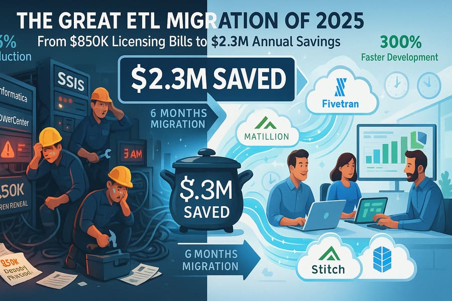
The Great ETL Migration: Why Companies Are Ditching Traditional Tools for Cloud-Native Solutions in 2025 A Fortune 500 manufacturing company…
Read More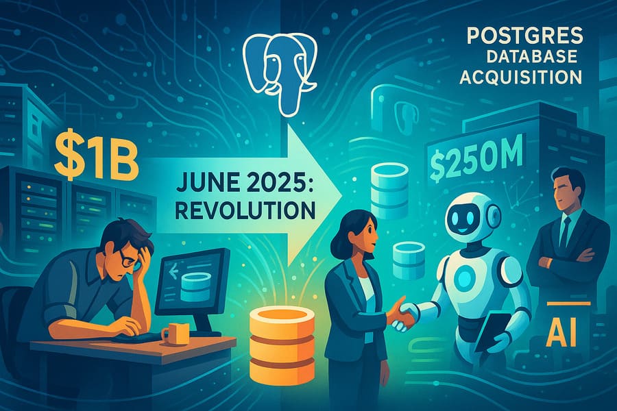
June 2025: The Month Data Engineering Got Seriously Competitive (And Why You Should Care) Remember when the biggest tech drama…
Read More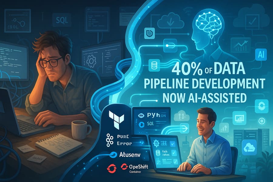
How AI Copilots Are Replacing Manual Data Pipeline Development: The 40% Revolution Transforming Data Engineering The data engineering landscape is…
Read More
IaC Horror Stories: When Infrastructure Code Goes Wrong A cautionary tale for data engineers venturing into infrastructure automation Picture this:…
Read More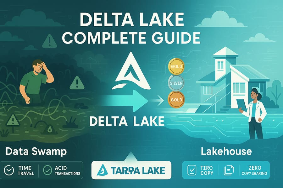
Building a Sub-Second Analytics Platform: ClickHouse + Delta Lake Architecture That Scales to Billions of Events Imagine querying 50 billion…
Read More
ClickHouse vs. Snowflake vs. BigQuery: Why the Delta Lake + ClickHouse Combo is Winning the Modern Data Stack Wars The…
Read More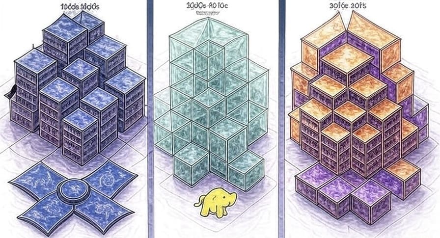
The Evolution of Data Architecture: From Traditional Warehouses to Modern Lakehouse Patterns – A Complete Design Guide for 2025 Introduction…
Read More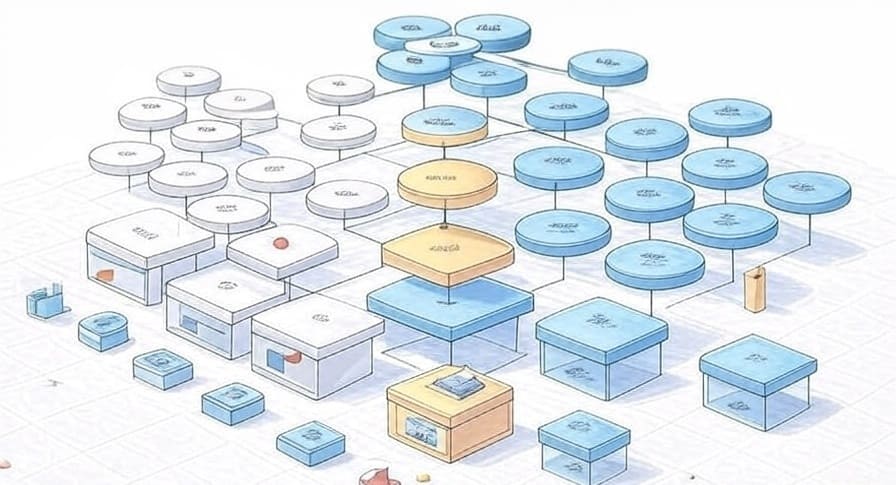
Data Modeling Concepts: Normalized, Star, and Snowflake Schemas – A Complete Guide for Data Professionals Introduction Data modeling forms the…
Read More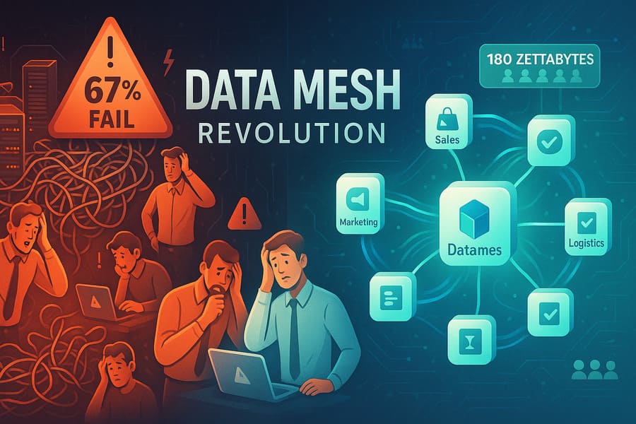
The Hidden Economics of Data Mesh: Why 67% of Implementations Fail and How Platform Teams Can Save $2M Annually Introduction…
Read More
The Hidden Psychology of ETL: How Cognitive Load Theory Explains Why Most Data Pipelines Fail Introduction Picture this: A senior…
Read More